A Bayesian parameter inference of the liquid culture model using Markov Chain Monte Carlo
A.1 Bayesian parameter inference
Bayesian parameter inference using Markov Chain Monte Carlo is an approach to curve-fitting that enables approximation of the probability distribution over model parameters given the observed experimental data. This section describes the selection of likelihood and prior functions used to estimate the posterior (Hogg, Bovy, and Lang (n.d.)).
The data available presents many options for defining the likelihood function. Many approaches to parameter inference for dynamical systems apply generative models to produce simulated data. At each parameter set sampled by the Markov process, the difference between the simulated and experimental values, or residual, is used to estimate the probability of the data given the sampled parameter set. The difficulty in taking this approach when dealing with a nonlinear dynamical system is that the distribution of residual values can be hard to determine or approximate. This is in part due to the fact that the residuals are not independent of one another. Consider, for instance, a generative model of the data that involves the numerical solution of ordinary differential equations that depends on the sampled parameters. Due to the continuity of the differential equations and, by assumption, the physical process that generated the experimental data set, large residuals are likely surrounded by large residuals. Instead of generating simulated data according to a sampled parameter set and the model equations, the approach we take here is to compute the residual of a self-consistency relationship derived from the model equations.
A.1.1 Defining the residual function
These self-consistency functions are derived from the differential equations described in Chapter 4. The equations governing protein expression include variables that represent intracellular concentrations. By rewriting these as equations relating the total quantities of each species, the equations then define an expected consistency between observable data, namely the derivatives of the fluorescence and optical density traces, and Hill functions. A residual calculation is performed by treating the Hill functions as the generative model describing the observed data.
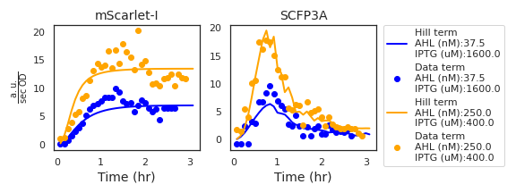
Figure A.1: The two plots show the Hill and Data terms based on data from two experimental wells and the maximum-posterior estimate for the liquid culture model parameters. The inducer concentrations from each well are included in the figure legend. While the Hill term values corresponding to the mScarlet-I channel are functions of simulated AHL transport and parameter values, those of the SCFP3A channel depend on observed density-normalized mScarlet-I fluorescence. Due to noise in measuring density-normalized fluorescence, the Hill term values of the SCFP3A channel appear less smooth than in the mScarlet-I channel.
Consider the differential equation that governs mScarlet-I expression, according to the liquid culture model:\[ \frac{\mathrm{d}R}{\mathrm{d}t} = x_R\,\mathcal{H}(\mathrm{A},\lambda_R, K_R) - (\rho_R + r_c (1 - \frac{c}{C_m})) R .\] Substitute the growth-rate dependent dilution term with the definition for the derivative of cell growth and simplify the notation by letting a time-varying function \(H(t)\) stand in for the production term: \[\begin{equation} \frac{\mathrm{d}R}{\mathrm{d}t} = H(t) - \rho_R R - \frac{\mathrm{d}c}{\mathrm{d}t} \frac{R}{c} . \tag{A.1} \end{equation}\] Now consider the relationship between the intracellular concentration of mScarlet-I, \(R\), and the total amount \(\hat R = cR\). Using the chain rule, we compute the derivative of the total mScarlet-I quantity: \[\begin{equation} \frac{\mathrm{d}\hat R}{\mathrm{d}t} = \frac{\mathrm{d}c}{\mathrm{d}t} R + c\frac{\mathrm{d}R}{\mathrm{d}t}. \tag{A.2} \end{equation}\] Using this relationship, we can substitute the terms for intracellular concentration \(R\) with those of the total quantity \(\hat R\) in Equation (A.1): \[\begin{equation} \begin{split} 0 &= H(t) - \rho_R R - \frac{\mathrm{d}c}{\mathrm{d}t} \frac{R}{c} - \frac{\mathrm{d}R}{\mathrm{d}t}, \nonumber \\ 0 &= H(t) - \rho_R R - \frac{1}{c}( \frac{\mathrm{d}c}{\mathrm{d}t} R - c \frac{\mathrm{d}R}{\mathrm{d}t} ), \nonumber \\ 0 &= H(t) - \rho_R R - \frac{1}{c}( \frac{\mathrm{d}\hat R}{\mathrm{d}t} ), \nonumber \\ 0 &= H(t) - \frac{1}{c}(\rho_R R + \frac{\mathrm{d}\hat R}{\mathrm{d}t} ). \tag{A.3} \end{split} \end{equation}\] Just as \(H(t)\) is a time-varying function, so to is the term \(D(t)=\frac{1}{c}(\rho_R R + \frac{\mathrm{d}\hat R}{\mathrm{d}t} ).\) These are called the Hill and Data terms, respectively, and examples are shown in Figure A.1. The residual is the difference between the two terms \[r = H(t) - D(t).\] As a result, the residual distribution can be approximated by the distribution of the Data terms. This same derivation is used to determine the definition of the residual for SCFP3A data, where the Hill term is a product of the three Hill functions describing IPTG activation, AHL activation, and transcriptional repression via Laci, and the maximal expression rate parameter \(x_S\).
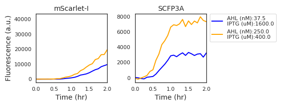
Figure A.2: Fluorescence data from two experimental wells with high expression activity show a marked delay in the initial accumulation of mScarlet-I fluorescence in comparison to SCFP3A fluorescence. Derivative estimates verify that there is no measured change in mScarlet-I fluorescence in the first half hour of data acquisition.
In the case of bicistronic LacI and mScarlet-I expression, we expect that the Hill functions vary in time only as the AHL concentration equilibrates between the cell volume and the growth media. This occurs rapidly (Kaplan and Greenberg (1985)). However, the data in Figure A.2 show a significant delay before the expression rate gradually ramps up to a peak and, finally, descending. The ramp up may be due to the long maturation time of mScarlet-I (roughly 66 minutes to 90% maturation) and the descent is likely due to slowing cell growth and protein production. This delay is less apparent in the SCFP3A fluorescence channel, perhaps due to its more rapid mautration (roughly 24 minutes to 90% maturation) (Balleza, Kim, and Cluzel (2018)).
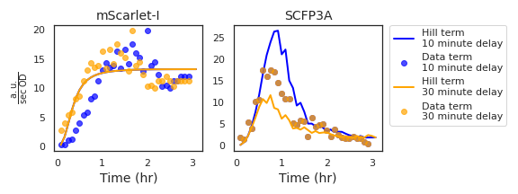
Figure A.3: Data from a single experimental well is shown here with two choices of mScarlet-I channel delay. The corresponding Hill and Data term values illustrate the effect of the delay parameter on how the residual is calculated. In the case of the mScarlet-I terms, the Hill term is left unchanged while the Data terms are moved backwards in time by the delay value. Data that fall into negative time are removed and replaced by resampling the same number of points from the end of the time series. The SCFP3A Data terms are unchanged while the Hill terms respond to the time-shifted density-normalized mScarlet-I fluorescence.
As the model does not consider maturation time or nutrient effects, an additional parameter is included while performing MCMC. This parameter represents impact of mScarlet-I’s maturation time on the observed fluorescence data and is demonstrated in Figure A.3. For a delay time \(t_d\), data from the mScarlet-I channel measured at time \(t_m<t_d\) is removed and the observation times of subsequent data are shifted backwards in time by \(\mathrm{Max}(t_m : t_m<t_d)\). To avoid favoring large delay times by removing data from the likelihood calculation, observations are added by resampling. When \(n\) observations are removed, \(n\) are resampled from the terminal \(n\) points of the time series.
A.1.2 Approximating the residual distribution
The residual distribution is difficult to approximate whenever its dependencies on model parameters, observation values, and other residuals are unknown (Hogg, Bovy, and Lang (n.d.)). One of the benefits of calculating the residual using the self-consistency relationships instead of simulated data is that each residual calculation represents an independent sampling of the residual distribution. When comparing data to a simulated ODE time series, on the other hand, the residuals at each point are not independent of one another. This section describes how the residual distribution of the self-consistency relationships were approximated.
The mScarlet-I channel Hill term is a function of AHL concentration, maximal expression rate \(x_R\), and Hill function parameters \(\lambda_R\) and \(K_R\) while the Data term depends both on the observed fluorescence and a single model parameter, \(d_r\). In determining the residual distribution, the contribution of uncertainty from the Hill term is ignored. It is assumed that understanding the distribution of Data term values is sufficient to describe the residual distributions. As the uncertainty in measuring Data term values results from the measurement process and sample-to-sample variability, it is natural to assume that both sources of uncertainty will result in a monotonic increasing relationship between the expected value and width of the distribution of Data terms. The task then becomes determining this relationship.
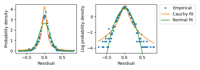
Figure A.4: Distribution of residual values from wells with Hill term values equal to 0. Empirical distribution values were determined through binning the \(n\) Data term values into \(2\sqrt{n}\) bins and calculating the normalized bin occupancy. The fit to a Normal distribution was perfomed by calculating the sample mean and standard deviation. The fit to a Cauchy distribution used the same sample mean. The Cauchy scale parameter was taken to be half of the sample standard deviation. The sample standard deviation here is 0.24.
This is accomplished by first characterizing the residual distribution when the Hill term is equal to zero, which corresponds to no mScarlet-I expression. In the case that both the Data and Hill terms are expected to be zero, the distribution of Data term values represents the uncertainty in measurement and sample preparation. Sample variability can only introduce uncertainty, therefore the distribution when the Hill term is zero corresponds to the minimum uncertainty in the residual distribution. Figure A.4 depicts the distribution of mScarlet-I channel Data term values recovered from experimental wells without any added AHL.
The distribution of residuals at higher Data term values was approximated by sampling the highest 4 Data term values from experimental wells grouped by AHL concentration. Data terms depend on a single model parameter that at this point is unknown. For the purpose of estimating the residual distribution, the a priori expected value of \(2\cdot10^{-4} /\mathrm{second}\) was selected. Data term values from the mScarlet-I channel reach a plateau after a few hours (see Figure A.1 ). By sampling values from the plateaus corresponding to different experimental wells, pooled according to inducer condition, the resulting distribution reflects both measurement residual and sample-to-sample variability. The sample means and standard deviations were computed for each pooled group of Data term values and plotted to determine the relationship between distribution width and expected value. Figure A.5 depicts the observed width - center pairs along with the scaling law implemented in the likelihood calculation.
To verify that the distribution scaling law appropriately described data from all ranges of Data term values, the data within each pooled group was rescaled according to the sample means and standard deviation as predicted by the scaling law. Following this, the data were collated and its empirical density function computed. The result, as shown in Figure A.6, appeared to be well-represented by a Normal distribution.
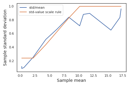
Figure A.5: Investigating the residual distribution in the mScarlet-I channel at high expression from liquid culture experiments. This plot of rescaled Hill and Data terms from high-expression samples suggests that the scaling law appropriately describes the residual distribution as mScarlet-I fluorescence increases. Data term values were rescaled according to the scaling law and an empirical density function was calculated. The empirical probability density function is plotted against fitted Normal and Cauchy distributions. This data set is much smaller than that of Figure A.4, so only \(\sqrt{n}/2\) equal-sized bins were used in calculating the empirical density function. The by-eye match between the empirical density values and the Normal distribution was the basis of selecting a Normal distribution using the scaling law in the likelihood calculation.
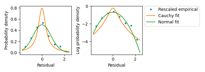
Figure A.6: Investigating the residual distribution in the mScarlet-I channel at high expression from liquid culture experiments. This plot of rescaled Hill and Data terms from high-expression samples suggests that the scaling law appropriately describes the residual distribution as mScarlet-I fluorescence increases. Data term values were rescaled according to the scaling law and an empirical density function was calculated. The empirical probability density function is plotted against fitted Normal and Cauchy distributions. This data set is much smaller than that of Figure A.4, so only \(\sqrt{n}/2\) equal-sized bins were used in calculating the empirical density function. The by-eye match between the empirical density values and the Normal distribution was the basis of selecting a Normal distribution using the scaling law in the likelihood calculation.
A similar approach was employed to determine the appriopriate scaling law for the SCFP3A residual distrubtion. Figures A.7 through A.9 show residual distributions and scaling law.
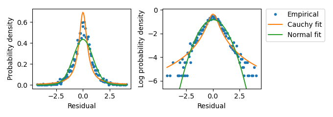
Figure A.7: Investigating the residual distribution in the SCFP3A channel at low expression from liquid culture experiments. Distribution of residual values from wells with Hill term values equal to 0. Empirical distribution values were determined through binning the \(n\) Data term values into \(2\sqrt{n}\) bins and calculating the normalized bin occupancy. The fit to a Normal distribution was performed by calculating the sample mean and standard deviation. The fit to a Cauchy distribution used the same sample mean. The Cauchy scale parameter was taken to be half of the sample standard deviation. The sample standard deviation here is roughly 1.
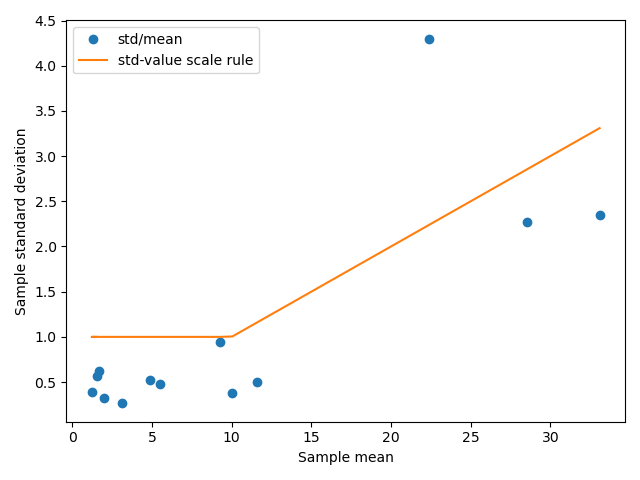
Figure A.8: Characterizing the scaling law for residual distributions in SCFP3A fluorescecne data from liquid culture experiments. This plot depicts in blue the sample means and standard deviations calculated of the Data term values, grouped according to AHL and IPTG concentration. The orange line depicts the scaling law used to define the residual distribution’s standard deviation.
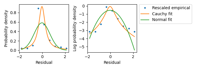
Figure A.9: Investigating the residual distribution in the SCFP3A channel at high expression from liquid culture experiments. This plot suggests that the scaling law appropriately describes the residual distribution when the Hill and Data terms are larger than zero. Data term values were rescaled according to the scaling law and an empirical density function was calculated. The empirical probability density function is plotted against fitted Normal and Cauchy distributions. Again, only \(\sqrt(n)/2\) equal-sized bins were used in calculating the empirical density function. The by-eye match between the empirical density values and the Normal distribution was the basis of selecting a Normal distribution using the scaling law in the likelihood calculation.
MCMC was performed using the emcee python package, making use of 1000 walkers and the kombine move selector (Foreman-Mackey et al. (2012), Farr and Farr (2015)). The chain was run for 10000 steps and the walker occupancy distrubtion appeared unimodal. Figure A.11 depicts the positions of the walkers at each iteration. The acceptance rate is well below the optimal for the dimensionality of the posterior distribution. This typically indicates that the walkers have discovered multiple local minima such that the move selector cannot produce a likely proposal. However, due to the proximity of these apparent local minima, the large number of walkers used, and the appearance of the marginalized posterior distributions, the chain is accepted as is. Furthermore, the authors of the emcee package note that many problems suffer from a vanishing acceptance rate, but that this is no cause for concern outside of applications in high-accuracy machining or involving life-or-death decision-making (Foreman-Mackey et al. (2012)). Outside of these cases, a chain with low-acceptance that surpasses 10 autocorrelation times can be considered a reliable approximation of the posterior distribution. Empirical cumulative density functions for each parameter are depicted in Figure A.10.
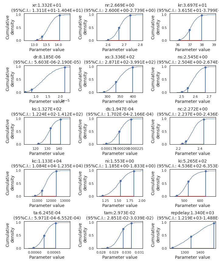
Figure A.10: Empirical cumulative density derived from the MCMC chain. Stem plots bracket the middle 95 centiles and mark the maximum estimated posterior parameter set between them.
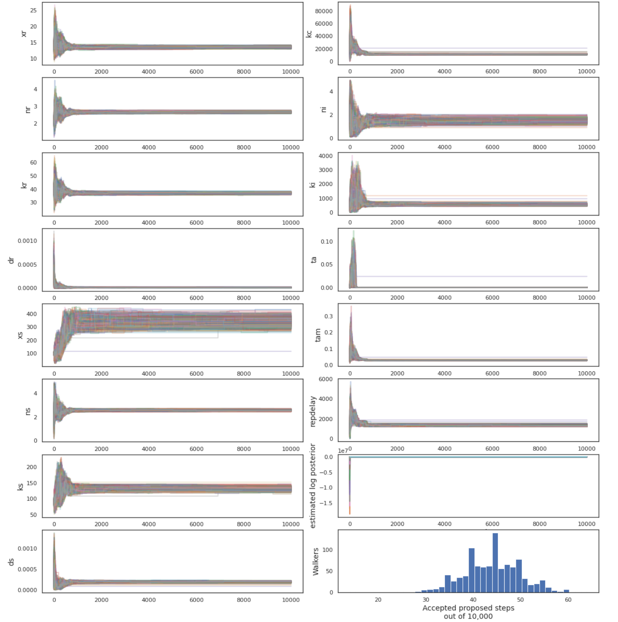
Figure A.11: Walker positions in parameter space over all iterations. Estimated log posterior values were calculated by the emcee ensemble sampler instance. The initial positions of the walker were selected from the a priori best fit, but all walkers quickly moved to a more likely region of parameter space.
References
Balleza, Enrique, J. Mark Kim, and Philippe Cluzel. 2018. “Systematic characterization of maturation time of fluorescent proteins in living cells.” Nature Methods 15 (1): 47–51. https://doi.org/10.1038/nmeth.4509.
Farr, B., and W. M. Farr. 2015. “Kombine: A Kernel-Density-Based, Embarrassingly Parallel Ensemble Sampler.” In Preparation.
Foreman-Mackey, Daniel, David W. Hogg, Dustin Lang, and Jonathan Goodman. 2012. “emcee: The MCMC Hammer.” Publications of the Astronomical Society of the Pacific 125 (925): 306–12. https://doi.org/10.1086/670067.
Hogg, David W, Jo Bovy, and Dustin Lang. n.d. “Data analysis recipes: Fitting a model to data *.” http://arxiv.org/abs/1008.4686v1.
Kaplan, H. B., and E. P. Greenberg. 1985. “Diffusion of autoinducer is involved in regulation of the Vibrio fischeri luminescence system.” Journal of Bacteriology 163 (3): 1210–4. https://doi.org/10.1128/jb.163.3.1210-1214.1985.