Chapter 4 Model development

4.1 Introduction

The time-lapse microscopy experiments presented in Chapters 2 and 3 demonstrated that amplifier cells can support communication between sender-receiver signaling pairs. The question then becomes can amplifier cells benefit communication within more complex consortia? While the amplifier cells succeeded in increasing the signaling distance of sender cells, the data make clear that the organization of consortia members, environment geometry, and timing are critical to its performance. The timing can be broken down into three phases. In the first phase, sender cells grow and accumulate synthase protein. During the second phase, the consortia density has increased to the point that sender cells can initiate a propagating wave through the amplifier cells. This propagation ends at the third phase, when cell growth and protein production slow down such that the amplifier cells cannot produce enough synthase protein to sustain signal transmission. Cells in a consortium will transition between these phases at different times, compounding the spatially heterogeneity of the consortium’s demographic patterning to the gene expression capacity.

This chapter walks through the development of a finite differences method (FDM) approach to simulating a reaction-diffusion model of sender-amplifier consortia. These simulations help to determine the applicability of amplifier strains to collaborative computations under the restrictions of the three phases outlined above. First, a set of ordinary differential equations (ODEs) describing the behavior of the amplifier strain in liquid culture is presented. While the goal is to simulate new engineered consortia in semisolid media, development begins with parameter identification on these ODEs using data from liquid culture experiments. These equations are adapted to a reaction-diffusion model and are supplemented with equations describing sender cell growth and signal release. While the gene circuit parameters inferred from liquid-culture experiments are maintained, microscope data are used to determine parameters governing nutrient-dependent growth and protein production. Finally, reaction-diffusion simulations of the sender-amplifier consortia are validated against experimental data described in Chapters 2 and 3 and then extended to predict the behavior of complex hypothetical consortia.

4.2 Parameter inference from liquid-culture experiments

4.2.1 Well-mixed Media Model

The experiments described in Section 2 produced the the data used to infer gene circuit parameters. We here describe the ordinary differential equations model for pulse-generator circuit behavior in liquid culture. The intention is for the model to capture the observed fluorescence dynamics using as simple a model as possible, not to make mechanistic inferences about hidden cell state variables. This liquid-culture model will then be adapted to a spatiotemporal PDE problem, where any simplifying assumption made at in the liquid culture model will facilitate the PDE model’s implementation and execution.

In the model, expression activation is modeled using Hill functions of the form \[\mathcal{H}(A,\lambda,K) = \frac{A^\lambda}{K^\lambda + A^\lambda}. \] In this form, the parameter \(K\) represents the IC50, the concentration of inducer chemical \(A\) which generates expression rate at half the maximal value, and the parameter \(\lambda\) controls how sharp the transition is from low to high output around the IC50 point. Lower values correspond to more gradual transitions and higher values. Protein quantity is also diminished through dilution as cells grow and divide. In the ODE, the protein concentration diminishes proportionally to the variable rate term \[ r_c (1 - \frac{c}{C_m}), \] where \(c\) is the cell density, \(r_c\) is the maximal cell growth rate, and \(C_m\) is the carrying capacity of the amplifier strain. Co-transcribed proteins are expressed proportionally to one another, the proportionality being dependent on their genetic context and RBS sequence. Identical LVA-ssrA degradation tags were appended to the coding sequences of the synthase, repressor, and reporter proteins to promote equal degradation rates, represented in the model as \(\rho\) with subscripts indicating the associated model species. As a result, for each protein-reporter pair, the expression rates are proportional and autodegradation rates can be treated as identical in the model. This permits the assumption that the ratio of co-transcriptional protein amounts is constant, a useful assumption when performing parameter inference (See Appendix A).

The combined production and degradation terms result in the governing equation of the model’s protein species. For LacI, the transcriptional repressor, that equation is \[ \frac{\mathrm{d}R}{\mathrm{d}t} = x_R\,\mathcal{H}(\mathrm{A},\lambda_R, K_R) - (\rho_R + r_c (1 - \frac{c}{C_m})) R, \] where \(x_R\) represents the maximal expression rate as a function of AHL, \(A\), and the Hill function parameters \(\lambda_R\) and \(K_R\). The synthase, CinI, is dependent on IPTG (model species \(I\)), AHL, and LacI concentration within the cell. Each chemical inducer is associated with a Hill function and the product of the three defines the production term. A decreasing Hill function \[ \mathcal{H}_{n}(R,\lambda,K) = \frac{K^\lambda}{K^\lambda + R^\lambda} \] is used to model the dependence of synthase expression on repressor protein concentration. LacI-mediated expression, however, is modulated by IPTG concentration. IPTG binds to LacI, preventing it from acting on operator regions in promoter sequences. To model the effect of IPTG, we scale the maximum synthase expression rate by an an increasing Hill function. This implies that the action of IPTG is independent of LacI concentration. While this is an unconventional approach to modeling this well-studied repression system, it was necessary to prevent simulations from producing small pulses in synthase concentration when AHL induction is low and IPTG is absent in order to match the observed circuit behavior. Under a more conventional set of gene regulation approximations, a simulation without IPTG and minor AHL would allow low levels of both synthase and repressor expression. The slow expression of repressor gives the simulated gene circuit time to accumulate a non-negligible amount of synthase, which would cause problems for parameter inference.

Letting \(x_S\) be the maximal expression rate of the synthase protein, the governing equation for CinI is \[ \frac{\mathrm{d}S}{\mathrm{d}t} = x_S\,\mathcal{H}(\mathrm{I},\lambda_I, K_I)\mathcal{H}(\mathrm{A},\lambda_S, K_S)\mathcal{H}_n(R,\lambda_C, K_C) - (\rho_S + r_c (1 - \frac{c}{C_m})) S .\]

According to these equations, cells should begin producing fluorescent proteins the instant AHL is added to the growth media. The data, however, show a delay between inducer spike-in and the response in fluorescence, as shown in Figure 4.1. AHL transport into the cell, transcription, translation, and fluorescent protein maturation all contribute to this delay. We will rely on equations governing AHL transport to enable the model to reproduce these delays. Other methods of accounting for this delay include introducing species representing mRNA and immature fluorescent reporters or employing delay-differential equations. Both approaches are common choices in the literature and could result in the observed delay. However, these would complicate the numerical solution of the finite-difference approximation of the reaction-diffusion PDE used to simulate microbial consortia described in Subsection 4.3. Therefore, the model relies a modified Fick’s first law to create these post-induction delays.

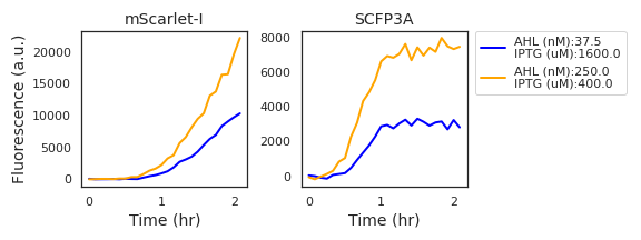
Figure 4.1: Fluorescence data from two experimental wells with high expression activity show a marked delay in the initial accumulation of mScarlet-I fluorescence in comparison to SCFP3A fluorescence.

AHL transport is modeled by Fick’s first law with a bounded transport rate, leading to the conditional equation

\[\begin{equation} \frac{\mathrm{d}A}{\mathrm{d}t} = \begin{cases} t_A(A_{\mathrm{Ext}}-A) & \text{if }\: |t_A(A_{\mathrm{Ext}}-A) | < t_{M}, \\ \mathrm{Sign}(A_{\mathrm{Ext}}-A)t_{M} & \text{otherwise.} \end{cases}. \end{equation}\]

The parameter \(t_A\) is the rate constant defining transport into the cell as a proportion to the difference in signal molecule concentrations between the external media and bacterial cytosol. Investigations into trans-membrane transport of AHL molecules have found that larger quorum sensing molecules rely on active transport. Applying an upper bound \(t_{M}\) to the transport rate is to consider saturation of the active transport proteins. The impact of transport on the external AHL concentration is ignored, as the volume fraction of the bacterial population is much less than the volume of the growth media. \(A_{\mathrm{Ext}}\), therefore, is a constant, equal to the concentration of AHL added at the beginning of an experiment. While the synthase could contribute to the concentration of AHL, we do not model this effect. As discussed in Section 2.2, increasing synthase expression did not result in increased mScarlet-I expression.

The full set of differential equations

\[ \begin{split} \frac{\mathrm{d}A}{\mathrm{d}t} &= \begin{cases} t_A(A_{\mathrm{Ext}}-A) & \text{if }\: |t_A(A_{\mathrm{Ext}}-A) | < t_{M} \\ \mathrm{Sign}(A_{\mathrm{Ext}}-A)t_{M} & \text{else} \end{cases}\\ \frac{\mathrm{d}R}{\mathrm{d}t} &= x_R\,\mathcal{H}(\mathrm{A},\lambda_R, K_R) - (\rho_R+r_c(1 - \frac{c}{C_m})) R \nonumber \\ \frac{\mathrm{d}S}{\mathrm{d}t} &= x_S\,\mathcal{H}(\mathrm{I},\lambda_I, K_I)\mathcal{H}(\mathrm{A},\lambda_S, K_S)\mathcal{H}_-(R,\lambda_C, K_C) - (\rho_S + r_c (1 - \frac{c}{C_m})) S\\ \frac{\mathrm{d}c}{\mathrm{d}t} &= r_c\,c\,(1 - \frac{c}{C_m}) \end{split} \] are applied as a generative model used during Bayesian parameter inference described in Appendix A.

4.3 Reaction-diffusion Model

The model described in the previous section was adapted to a reaction-diffusion model to describe the behavior of cells growing on the surface of agarose pads. This simulation approach was adapted from one used in a related project (Doong, Parkin, and Murray (2017)). A reaction-diffusion model is a system of partial differential equations of the form \[ \partial_t u = D \nabla^2 u + f(u) .\] The function \(f\) is called the reaction term; it describes the dynamics resulting from interactions between model species. The diffusion term is \(D\nabla^2u\), which confers linear, isotropic diffusion at rates \(D_{i,i}\). \(D\) is an \(n\times n\) real-valued matrix and \(u\) is a vector of \(n\) terms.

Evolution equations from the well-mixed media model become the components of the reaction term \(f(u)\), with a few modifications. Instead of logistic growth, the bacterial division rate varies with the local value of a model species representing nutrient concentration. Both cell growth and protein production depend on nutrient availability. Just as the relationship between chemical inducers and protein expression rate is defined by a Hill function, the nutrient species scales cell growth and protein production generally; an approach that is adapted from Liu et al. (2011). Each evolution equation governing these species includes a production term that is scaled by a \[\mathcal{N}(t,x,y) = \mathcal{H}(n(t,x,y), \lambda_n, K_n),\] a term representing nutrient availability. While protein production and cell growth depend on nutrient availability, only cell growth actually consumes nutrients. This feature is anchored in the assumption that the metabolic investment in the synthetic circuit’s proteins is minor compared to host functions.

The reaction terms for the model species representing the sender and amplifier strains are \[ \begin{split} \frac{\mathrm{d}C_{\mathrm{sender}}}{\mathrm{d}t} &= r_c\,\mathcal{N} C_{\mathrm{sender}},\nonumber \\ \frac{\mathrm{d}C_{\mathrm{pulser}}}{\mathrm{d}t} &= r_c\,\mathcal{N} C_{\mathrm{pulser}}\nonumber \\ \text{and the resulting change }&\text{in nutrient concentration is defined by}\\ \frac{\mathrm{d}n}{\mathrm{d}t} &= - \rho_n\,( C_{\mathrm{sender}} + C_{\mathrm{pulser}} )\; \mathcal{N}, \nonumber \\ \end{split} \] where \(\rho_n\) is the nutrient consumption rate. The initial condition of the nutrient concentration is 100, uniform over the simulation space. 100 is a value selected out of convenience and the species is unitless. Nutrient and cell density are exchanged at a rate of \(r_c/\rho_n\), meaning the total amount of cell produced during a simulation is bounded by \(100 r_c / rho_n\).

The reaction terms corresponding to the protein species have a production and degradation term, just as in the well-mixed media model. Degradation terms, however, must be adapted according to the growth model. In place of the logistic function is the \(\mathcal{N}\) scaling term and a masking function to limit protein expression to the appropriate regions. Masking is accomplished by applying a Heaviside function on the concentration of cell species, biased negatively by a small bias term \(\epsilon_c\). When simulations incorporate non-zero diffusion rates for the cell species, cells may invade nearby space. Masking ensures protein expression occurs only in regions occupied by cells of the correct identity. The small bias ensures that, in the case of linear diffusion, the rapidly expanding cell mass does not result in an equally rapid expansion of protein expression. It is a well-known fact from transport theory that linear isotropic diffusion results in infinite range expansion; any local perturbation of a continuously-valued, diffusing species instantly produces a global effect. While this is not the case in a finite difference scheme, the range does increase with each time step and the bias term prevents expression from regions of negligible cell concentration. With these alterations, the reaction terms governing protein species evolution are

\[ \begin{split} \frac{\mathrm{d}R}{\mathrm{d}t} &= (x_R\,\,\mathcal{H}(\mathrm{A},\lambda_R, K_R) \Theta(C_{\mathrm{pulser}}-\epsilon_c) - r_c R)\mathcal{N} - \rho_R R \nonumber \\ \text{for the }&\text{repressor species and}\\ \frac{\mathrm{d}S}{\mathrm{d}t} &= \left( x_S\,\mathcal{H}\left(\mathrm{A},\lambda_S, K_S\right)\mathcal{H}_-\left(R,\lambda_C, K_C\right) \Theta\left(C_{\mathrm{pulser}}-\epsilon_c\right) +\right . \nonumber\\ &\qquad \left. x_O \,\Theta\left(C_{\mathrm{sender}}-\epsilon_c\right) -r_c S \right)\mathcal{N} - \rho_S S \nonumber \end{split} \] for the synthase species. Finally, AHL synthesis is emitted at a rate proportional to the synthase quantity at a location and degrades according to the autodegradation term \(\rho_A\): \[ \frac{\mathrm{d}A}{\mathrm{d}t} = x_a\,S\,(C_{\mathrm{pulser}} + C_{\mathrm{sender}}) - \rho_A A \;. \]

The finite difference method (FDM) is an approach to approximating partial differential equations using difference equations. These difference equations are designed to approximate the PDE system on a set of grid points, in this case over the space and time variables. In this model, the difference scheme applies second-order second central difference equations to approximate the second-order spatial derivatives. The grid used in the FDM scheme is conceptually similar to a compartmentalization of the agarose arena into cubic chambers. The model species take on a single value within each chamber and evolve according to the ODE model equations and diffusion. For a parameter set \(p\) and state vector \(u\), the finite-difference approximation to the reaction-diffusion system results in the difference equation \[ \frac{u_{n+1}-u_{n}}{\Delta t}= \frac{1}{{\Delta x} ^2}A(p)\cdot u_n+f(u_n;p).\] \(A(p)\) is a matrix that applies the second-order central differences approximation of the Laplace operator, resulting in difference equations of the form \[\begin{equation} \begin{split} \mathcal{L}(u(t,x,y)) = \sum_{\substack{1 = \lvert(i,j)-(x,y)\rvert\\ (i,j) \in \mathrm{P}}} \frac{1}{\Delta x^2} \big(u_{i,j} - u_{x,y} \big) \end{split} \;\;\; \tag{4.1} \end{equation}\] that describes diffusion at each position \((x,y)\) given the values at neighboring positions in the grid \(P\). The finite difference schemes applied to this problem take equally spaced grids in all spatial dimensions. In Equation (4.1), there are two spatial dimensions, so \(\Delta x = \Delta y\). In the case of linear, isotropic diffusion, the matrix \(A(p)\) is a constant, band matrix. The band structure in \(A(p)\) applies the second-order central differences while \(D\), from the PDE, is diagonal and scales the Laplacian terms according to their diffusion rates. The matrix \(A(p)\) also provides no-flux boundary conditions to ensure diffusing species do not escape the agarose pads at its boundaries. Note that the size of matrix \(A(p)\) is \(n\times n\) for \(u_n \in \mathbb{R}^n\); though the simulated arena is two-dimensional, the values of the model species over the two-dimensional spatial grid is represented as a vector and the diffusion operator as a two-dimensional matrix.

4.3.1 Accounting for out-of-plane diffusion

It would be convenient to find a difference scheme that can produce simulated data that is similar to experimental observations without explicitly tracking AHL concentration within the interior of the agarose pad. However, scaling laws described by Dieterle et al. (2020) suggest that the most natural treatments, either of an infinitely tall pad or a negligibly tall pad, are not appropriate given the similarity in the measured propagation velocity (in the area of 1-2 mm/hr) and the height of the pad (roughly 1.5mm). Here, the agarose pad organization described in Section 2.3 is applied to determine the impact of AHL diffusing out of the plane of interest through simulation.

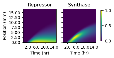
Figure 4.2: The two plots depict simulated protein quantities (in arbitrary units) along the sender-amplifier consortium at each simulation time step. Quantities are determined by multiplying the model species of cell density by those representing intracellular protein concentrations. The intensity values depicted in the heatmaps are normalized to the maximum value in each image.

The organization of strain components on the agarose pads applied in Section 2.3 to investigate signaling propagation along one dimension was designed to minimize rate at which diffusion carried AHL away from consortium cells. Sender strains were separated from their consortium partner strains, either amplifiers or reporters, and isolated to a narrow region at one end while their partner strain occupied the larger portion. As a result, the experimental setup was symmetrical in one dimension. Thus, simulations of this setup can consider only two dimensions, one in the direction of signal propagation and one perpendicular to the surface the cells live in.

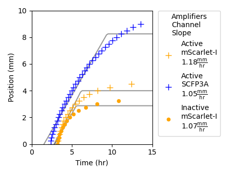
Figure 4.3: This plot shows the propagating front of signaling activity as represented by the quantities of repressor and synthase species. To determine the position of the signaling front, a threshold was applied to the fluorescence data presented in Figure 4.2. The points depicted in the plot correspond to the position farthest from the sender population that surpasses the threshold value at each time step. Threshold values were determined by the Otsu thresholding method. Propagation velocities and maximum signaling distances were determined by fitting a line of the form \(\text{Min}(at+b,c)\), where \(t\) is simulation time, \(a\) is velocity, and \(c\) is maximum calling distance, were fit by least squares.

Simulations of the model described in Section 4.3 were performed that matched the cell patterning and agarose dimensions applied described in Section 2.3. The simulation region described a surface 2mm high and 24mm long, matching the dimensions of the agarose pads used during time-lapse microscopy experiments. In the initial data used for numerical solution of the initial value problem \[ u_{n+1} = A(p)u_n+f(u_n), \] cells were confined to the bottom row of a two-dimensional grid that spanned the pad height with grid spacing \(\Delta x = \frac{1}{16}mm\). Diffusion was considered only for the model species representing AHL. Due to the uniform cell occupation across the pad length, no spatial variation could occur in nutrient or cell density. Diffusion rates for the protein species were likewise set to zero. The simulation ran for a simulated time of 15 hours.

Figure 4.2 depicts protein quantities over the layer of cells and time grid from a simulated sender-amplifier consortium. Just as in the experimental data depicted in Figure 2.6, after a period of a few hours, the amplifier cells respond to AHL secreted by the near by sender cells (which occupy the grid positions between 0 and -4mm) and produce a propagating front of signaling activity that travels away from the sender population. The position of this signaling front over time is shown in Figure 4.3. The front produced by the simulated consortia travels farther and slightly slower than the experimental consortium (see Figure 2.7). However, the three phases of pulse propagation remain: pre-initiation growth, constant-velocity propagation, and nutrient depletion, and the behavior is remarkably similar considering the model parameters were identified from data generated by liquid culture experiments.

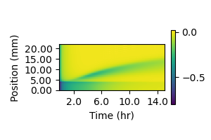
Figure 4.4: The difference between AHL concentrations in the cell layer and the layer immediately above it was calculated at each gridpoint within the cell layer, then divided by the value in the cell layer. The value in the cell layer was subtracted from the value in the higher layer. Negative values indicate a concentration drop in the out-of-plane direction, which results in out-of-plane diffusion. Values closer to zero indicate a flat profile where diffusion has less of an impact. The interface between the sender and amplifier regions is at 4mm, with sender cells below that line and amplifier cells above it.

Figure 4.4 shows the concentration drop in the out-of-plane direction, measured at each grid point in the cell layer. The more-negative values coincide with the synthase peaks in Figure 4.2, while the concentration profile everywhere is significantly less steep. This suggests that, as might be expected, out-of-plane diffusion is most significant near isolated, high-AHL emission regions and at the leading edge of the propagation front in particular. Away from these areas, diffusion smooths the out-of-plane concentration gradient and reduces the impact of diffusion along that vector. A reasonable approach to capturing the effect of out-of-plane diffusion without explicitly modeling signal transport within the interior of the agarose pad, therefore, would be reducing the expression rate of synthase protein or the synthesis rate of AHL. This reduction in expression rate accounts for the quantity of signaling molecule that is effectively sequestered in the interior of the pad by diffusion. This is more appropriate account for out-of-plane diffusion by increasing the autodegradation rate, which would lead to rapid concentration declines even away from high-emission regions where the out-of-plane diffusion rate should be small. One unrealistic result of this assumption is that it cannot account for the gradual accumulation of signaling molecules in high-synthesis regions. As seen in Figure 4.4, the concentration gradient over the sender cell population grows more shallow over time as signaling molecules accumulate above it. As this occurs, AHL accumulation within the cell layer will accelerate. However, this takes place well behind the propagating signaling front and has little impact on it. In order to capture the impact of out-of-plane diffusion at the leading edge of the propagating signaling front, the simplest appropriate adjustment was made: reducing the protein production rate of the sender synthase and the signal synthesis rate by half.

4.3.2 Finite difference scheme for growing microbial consortia in two dimensions

The purpose of developing this model of cell-cell communication within microbial consortia is to accurately reproduce observations made during time-lapse microscopy experiments and then extend its use to hypothetical consortia. These data show heterogeneous responses in fluorescence and growth at the sub-millimeter level. It is critical to determine whether these observations are natural consequences of the well-characterized growth and synthetic gene circuit models; if not, then our understanding of the synthetic consortia is insufficient to extend use of this model to more complicated consortia.

Unfortunately, the PDE model includes processes that proceed at drastically different time scales. This can make numerical solution problematic. It was the case that applying common general-purpose numerical solvers for stiff problems, such as Runge-Kutta 4(5) and LSODA, failed in integrating the nutrient-dependent growth model combined with the cell-cell signaling circuit with spatially heterogeneous microbial consortia. A fixed-step numerical integration method was therefore developed. While generally less computational efficient and accurate than variable time step methods, fixed-step methods can be customized to satisfy a priori accuracy constraints and guarantee completion of the requested integration. This subsection describes the fixed-step operator-splitting approach used in simulating complex, growing consortia on 2D surfaces.

It is likely that the “stiffness” at issue in this problem arises from the expanding microcolonies and the masking performed to restrict protein production to grid points that are sufficiently dense in cells. By splitting the system evolution into two steps and calculating the effect of the diffusion and reaction terms separately, each can be efficiently calculated according to their different time scales.

The diffusion step, due to the linearity of its differential operator, can be efficiently resolved using a second-order implicit method that ensures good performance while maintaining a relatively large fixed time step to speed integration. Relative to the diffusion term, the reaction term is both non-linear and more difficult to apply to an implicit approach. Instead, the reaction contribution is calculated using a simple explicit form, iterated several times over a smaller time step.

The diffusion step is performed by a Crank-Nicholson step. First, the diffusion step is proposed as an implicit difference equation \[ \tilde u_{n+1,i} = u_n + \frac{\Delta t}{2}A(p)(\tilde u_{n+1,i}+u_n) \] and is then rearranged to form the matrix equation \[ (I-\frac{\Delta t}{2}A(p))\tilde u_{n+1}=(I+\frac{\Delta t}{2}A(p))u_n\,, \] which permits approximation of the mid-step value \(\tilde u_{n+1,1}\) from the known value \(u_n\). Python scripts executing the simulation use SciPy’s generalized minimum residual method to quickly approximate the value of the unknown. Following this, the mid-step value \(\tilde u_{n+1,1}\) is used as the initial data for a series of forward Euler steps of the form \[ \tilde u_{n+1,i+1} = \frac{\Delta t}{4}f(\tilde u_{n+1,i}) + \tilde u_{n+1,i}\] that employ a time step \(\Delta t / 4\). The forward Euler steps are repeated four times to match the time step taken during the diffusion calculation, resulting in the final step value \(\tilde u_{n+1,5}=u_{n+1}\) at the completion of the time step. The time step for the implicit portion is selected according to the constraint \(\Delta t < \frac{\Delta x ^2}{6 D_a}\) to prevent oscillations in the diffusion step.

All model species have positive diffusion coefficients in the linear diffusion operator \(A(p)\). While E. coli can engage in random walks through flagellar motion and modeled as such using linear diffusion, the bacteria under the agarose pad move only as the result of crowding and pressure from microcolony formation. Nonlinear diffusion equations such as the permeable membrane equation would be a more appropriate descriptor of cell movement in this scenario. This is not pursued here, as linear diffusion enables more efficient integration. The nutrient-based growth model, however, achieves a similar range expansion effect that is achieved by slow diffusion of nutrient and cell species. While linear diffusion results in an immediate response across the spatial domain in the PDE, the low diffusion coefficients of nutrient and cell species creates a sharp transition from high to low density at the edge of cell-occupied regions.

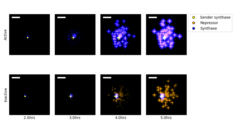
Figure 4.5: Simulations of sender-amplifier and sender-reporter consortia were performed, designed to recreate the experiments described in Chapter 3. The two rows of images show protein amounts from the sender-amplifier (Active) and sender-reporter (Inactive) consortia at selected time points. Protein concentrations are represented in the false-color images according to their identity and their associated cell type. Black indicates absence, and brightness correlates with quantity. A color key is indicated by the figure legend. The isolated point in the frames corresponding to 2 hours is the location of the single sender microcolony. Scale bar is 100\(\mu\)m.

Using this finite difference scheme and operator-splitting approach to time stepping, simulations were performed to match the conditions present in the experiments described in Chapter 3. Selected images representing the simulation state are depicted in Figure 4.5. The spatial grid in the scheme had \(\Delta x =\frac{1}{16}\)mm over a region \(9\text{mm}\times9\text{mm}\) and a Crank-Nicholson timestep of \(\Delta t = 3\)seconds was applied. Initial cell data were sparse boolean arrays, where the small number of high-density grid points were selected randomly from a \(0.7\)mm disk at the center of the spatial domain. For each simulation, a single high-density sender position was selected and 100 high-density amplifier or reporter positions were selected. The integration proceeded for 18000 time steps such that the time grid spanned 0 to 15 hours. Ten such simulations were performed for each consortium.

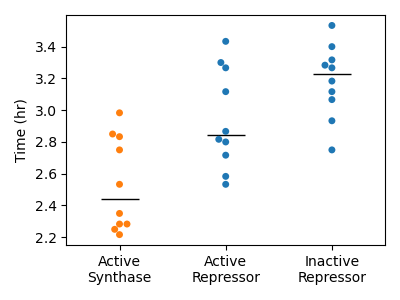
Figure 4.6: Response times observed in simulation. Each point represents the time at which the first reporter or amplifier grid point value crossed a threshold value. Threshold values were determined for each protein species by applying the Otsu method to the values generated from sender-amplifier consortia simulations. The black horizontal lines indicate the sample median.

While the simulated sender-amplifier consortia exhibit a marginally more rapid response to signals originated by the sender population than the sender-reporter consortia, the simulated consortia generally appeared to respond more rapidly than observed in experiment. Figure 4.6 shows the response time values calculated for each simulation. Compared to the analogous plot of experimentally observed response times in Figure 3.2, the simulated consortia activate in roughly in roughly half the time. Simulated sender-reporter consortia, where signal amplification is inactive, also showed a significant response. This can be seen in Figure 4.5, where the images in the “Inactive” row show a clear response near the sender colony that is absent from the experimental data in Figure 3.1. In contrast, experimental data showed almost no reporter activity. This suggests that the adjustments described in Section 4.3.1 did not sufficiently account for the impact of out-of-plane diffusion in this scenario. In order to improve this model’s ability to accurately recreate experimentally observed phenomena, the parameters controlling synthase expression in sender cells and synthase activity rate could be fit to the model data.

4.4 Evaluating the benefit of amplification in hypothetical consortia

Simulations were designed to apply the inferred parameters governing cell growth, sender activity, and amplifier activity to predict the behavior of hypothetical consortia to scenarios matching the growth and diffusive contexts described in Chapter 3: a consortium growing within a disk of 0.7mm diameter on an agarose pad 4.5mm by 4.5mm by 2mm. The consortia applied to these simulations express cell-cell signaling and transcriptional programs selected to explore the potential for collective decision-making in random founding cell patterns and spatiotemporally heterogeneous sender activity.

4.4.1 Chained sender-receiver cascade

The first consortium assayed is a chained sender-receiver cascade. Like the party game “telephone”, a cascade is initiated by one strain of sender cells secreting signals that are received by the next strain in the chain. This population then expresses synthase protein as activated by the initial signals, producing signal molecules that activate the following component of the chain. In total the chain contains five strains, the initiator and four subsequent chain components. Added to these chained sender-receiver relationships are amplifier cells that are triggered by each of the sender-receiver signaling species to emit a pulse of the same species. Figure 4.7a) conceptually represents this consortium structure, though not the founding cell patterning. The composition of these simulated consortia vary over the ratio of cascade cells to amplifier cells as well as toggling the amplifier cells between inactive, in which case they act as bystanders, or active amplifiers for all sender-receiver interactions. Varying the composition in this manner allows for the investigation of the relative benefit of amplifier cells as the cascade cells increase in density. Figure 4.7c) suggests that, with or without amplifier activity, the chained cascade produces negligible activity past the first interaction. However, the amplifiers succeed in boosting that response in all cases. This is likely due to nutrient depletion, which appears to enforce a time limit on effective consortium-wide communication at the simulated arena size, simulation time, and the assumption of an infinitely-deep diffusive environment.

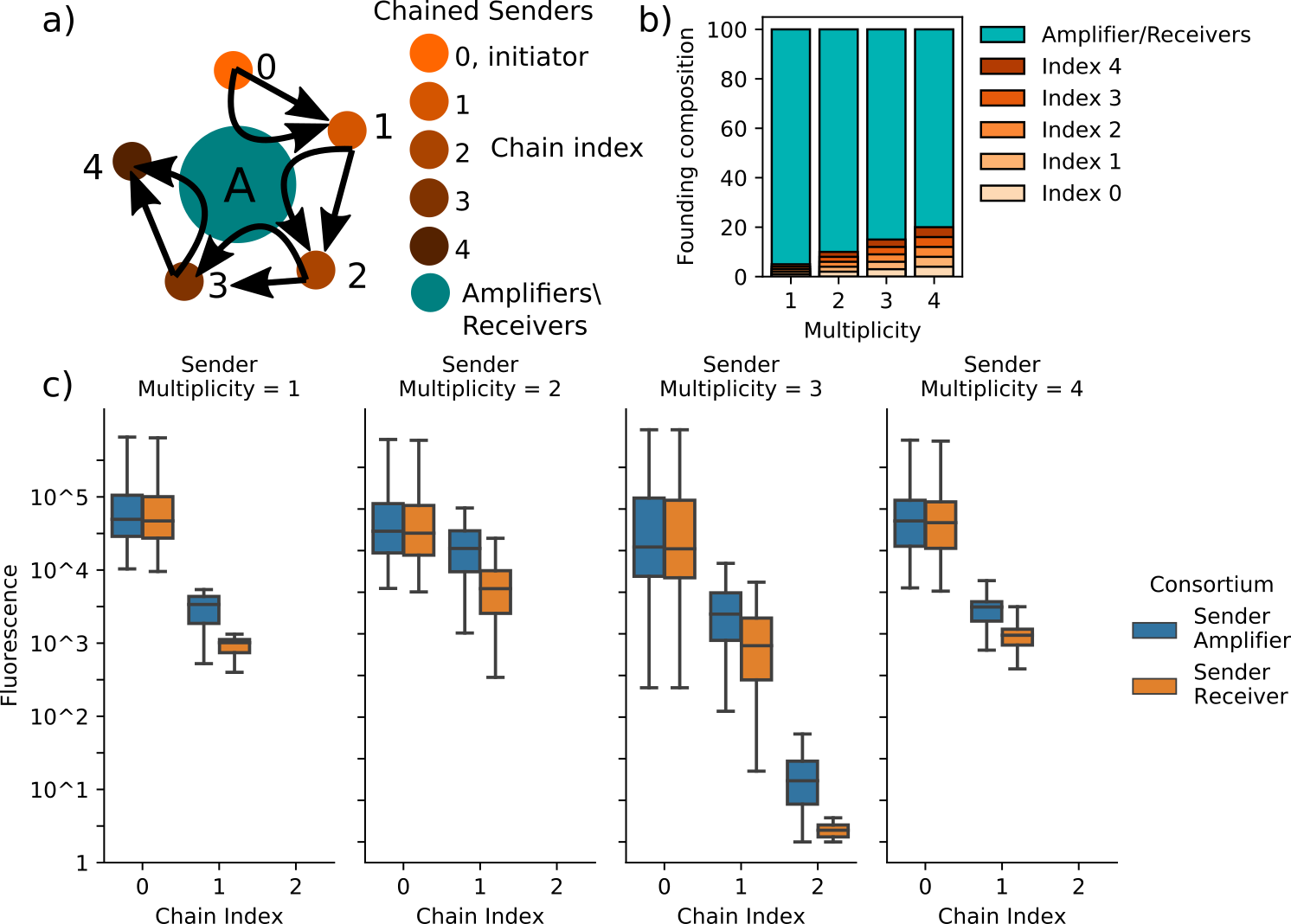
Figure 4.7: Hypothetical consortia composed of amplifiers/receivers and chained sender cells are simulated to evaluate how amplifying cell-cell signaling can benefit information propagation. (a) depicts a schematic representing the cell-cell signaling relationships represented in these simulations. The chained senders are connected by unidirectional, sender-receiver relationships in which chain index \(i\) emits signal molecules that activate synthase expression in chain index \(i+1\). The index 0 population are constitutively active. Each sender-receiver relationship employs unique, orthogonal signaling species Amplifiers, however, can amplifify the signaling activity at each index. Simulations vary the bystander cells’ status as amplifier or receiver and the composition of the founding consortia populations, which is described in (b). Sender multiplicity is the number of founding cells of each of the sender populations. Because the founding population is set at 100 individuals, higher multiplicity reduces the total number of amplifier/receiver cells in the founding population. The benefit provided by amplification is measured by comparing the maximum synthase amount in each sender population achieved during simulations including either amplifiers or receivers as partners to the chained senders. Receivers do not respond to signaling activity, but they occupy space and consume nutrients. (c) depicts, in boxplots, the distributions of sender activity at each index of the sender chain obtained over ten simulations of each consortium. Simulations of chain/amplifier and chain/receiver consortia utilize the same initial conditions such that the comparisons of the distributions are not confounded. In all assayed conditions, utilizing parameters governing gene networks and cell growth in B.1, the amplifiers increase the response in chain indices greater than 0. However, the response in all multiplicities except 2 is significantly diminished in comparison to the constitutively-active index 0 senders and the response from chain indices greater than 1 is negligible in all cases. Together, these data suggest that even with amplifier cells, a chained signaling cascade between minority populations is unlikely succeed past a single step.

4.4.2 Coincidence detector

The second consortium investigated was composed of amplifiers (or receivers when inactive), two sender populations, and a receiver. Simulating this consortium sheds light on how amplifying cell-cell signaling can benefit consensus in an environment of spatially heterogeneous chemical signals. In this scenario, the senders stand in for components of a deployed consortium that alert the community to environmental events to which they are uniquely sensitive. Receivers respond to the simultaneous presence of signals from both sender cells, which can also be amplified by the amplifier strain. Simulations are performed that apply varied pulses of activity from the sender populations. The success of the communication strategy is evaluated on the basis of simulated fluorescence from the receiver population. A conceptual summary of this consortium and results provided in Figure 4.8a). The results show an unexpected pattern of receiver response in which the strongest activity arose from simulations with sender pulse timings at time 2 and 5 hours with a pulse width of 4 hours. This implies an overlap in both pulses of 1 hour, relatively short compared to other simulations that produced overlaps of 2 or 3 hours. While increasing the overlap time naturally results in more receiver activity, it appears that separating the initiating times of the two sender populations has a greater benefit. The reasons behind this are not clear and further investigation is required before arriving at conclusions. It is clear that the time-varying nutrient availability and spatial patterning is a key determinant of both the effectiveness of cell-cell communication within consortia executing complex programming and the benefit provided by amplifier strains.

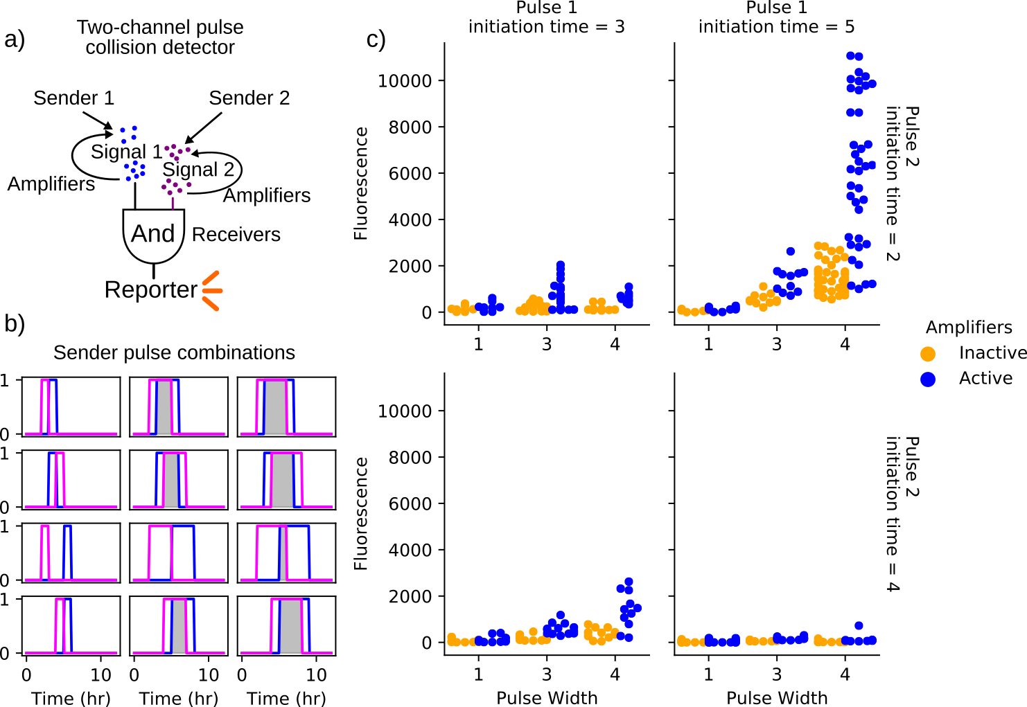
Figure 4.8: Outline and results of the coincidence detector consortium. (a) depicts a schematic representing the cell-cell signaling relationships represented in these simulations. The two sender populations initiate signaling through the release of diffusible signaling chemicals. Amplifiers, when active, are triggered by the sender populations to contribute to the local concentrations of these chemicals in a pulsatile fashion. The receiver population produces a fluorescent output in the presence of both signaling molecules. Simulations vary the timing and duration of synthase expression within the sender populations as shown in (b). Simulations span 12 hours. Gray-shaded regions indicate overlapping synthase expression within the sender populations. Plots in (c) show the maximum pixel values within the receiver population obtained over three simulations of each sender-emission pattern. Each of these three iterations employs a different random spatial patterning of the founding population, which is composed of a single founder of each of the sender and receiver strains and 100 amplifier/bystander cells. These random initial conditions are repeated for consortia with active and inactive amplifier cells such that active/inactive cases can be compared directly. In all assayed conditions, utilizing parameters governing gene networks of sender, amplifiers, and receivers as well as cell growth in B.1 and use the same arena and consortia geometry as in 4.5. The simulated receiver fluorescence indicates the degree to which the population receives input from both sender cells. All conditions show a greater average response in the receiver population when amplifiers are active. However, only the simulations in which one pulse initiates at 2 hours and the other at 5 hours results in significant expression. This is likely a result of the time-varying nutrient availability and suggests the relationship between event timing and response is non-trivial and not intuitive. Further exploring the spatiotemporal dynamics of nutrient availability in simulation requires more experimental data capturing these effects in order to be predictive.

References

Dieterle, Paul B, Jiseon Min, Daniel Irimia, and Ariel Amir. 2020. “Dynamics of diffusive cell signaling relays.” eLife 9. https://doi.org/10.7554/elife.61771.

Doong, Joy, James Parkin, and Richard M. Murray. 2017. “Length and time scales of cell-cell signaling circuits in agar.” bioRxiv, 1–19. https://doi.org/10.1101/220244.

Liu, Chenli, Xiongfei Fu, Lizhong Liu, Xiaojing Ren, Carlos K. L. Chau, Sihong Li, Lu Xiang, et al. 2011. “Sequential establishment of stripe patterns in an expanding cell population.” Science 334 (6053): 238–41. https://doi.org/10.1126/science.1209042.