C Inferring Parameters Governing Cell Growth in Semi-solid Media

C.1 Introduction

The growth process of cells in semi-solid media is different from growth in liquid culture and therefore requires different treatment within a model. In a diffusive environment, such as an agarose pad, cells deplete local nutrient concentrations while dividing exponentially. Following this depletion, microcolonies grow at a reduced rate, consuming nutrients as they diffuse away from unoccupied or more sparesly occupied by cells. Furthermore, cells divide more slowly as a result of contact inhibition (Payne et al. (2013), Cao et al. (2016)).

Disentangling the various mechanisms affecting division rates in semi-solid media is an active area of research that is beyond the scope of this work. The goal here is to apply a simple model describing cell growth that accurately reflects the empirical growth curves observed during time-lapse microscopy experiments. To do so, a model of cell growth in a diffusive environment is selected that can, under different parameter choices, reflect the range of expected growth behaviors. Then, parameters are selected to minimize the difference between experimental and simulated data.

C.2 Growth model

The model of cell growth used in the finite-differences approximation simulations was based on the work of Liu et al. (2011). In this model, the division rate at a position is related to the value of a nutrient species by a Hill function of the form

\[\begin{equation} \frac{\partial_t c}{c} = r_c \frac{n^{\lambda_n}}{n^{\lambda_n} + K_n^{\lambda_n}} \end{equation}\]

As noted in Chapter 2, the shorthand

\[\begin{equation} \mathcal{H}(a,n,K) = \frac{a^{n}}{a^{n} + K^{n}} \end{equation}\]

is used for Hill functions.

At the beginning of a simulation, the nutrient species is equal to 100, a nondimensional quantity. This is simply for convenience in notation; a value of 100 indicates 100% nutrient availability. Nutrients diffuse freely within the no-flux boundaries of the simulation. The rate of cell growth is proportional to the rate at which nutrient is consumed. Nutrient quantities are therefore diminished at a rate proportional to the Hill function as well. The model parameter \(\rho_n\) defines this proportionality. The two differential equations comprising this nutrient-based model are

\[\begin{equation} \begin{split} \partial_t n &= D_n \nabla^2 -\rho_n \mathcal{H}(n,\lambda_n,K_n)\\ \partial_t c &= r_c \mathcal{H}(n,\lambda,K_n). \end{split} \end{equation}\]

C.3 Dataset

A set of time-lapse microscopy experiments were performed to capture the growth behavior of E. coli cells on agarose pads. Competent cells of the strain JS006 were transformed with a plasmid conferring constitutive expression of the mScarlet-I fluorescent protein. These cells were deposited onto agarose pads using an acoustic liquid handler. A variety of growth contexts were implemented that varied in both the seeding population density and shape, the position of the colonies on the agarose pad, and size of the agarose pad. Images depicting these contexts are shown in Figure C.1.

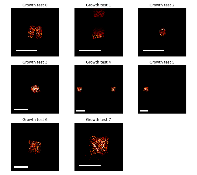
Figure C.1: The images in each plot show the fluorescence micrographs of the different agarose pad growth contexts. The images show the size and position of the cells on the square agarose pads of varying sizes. While the images were collected with a spatial resolution of 0.89 \(\mu\)m, these images were downsampled by a factor of 64 in order to match the spatial resolution of the simulated data. Scale bars in each image are 4mm.

Seeding shapes were square patterns of Echo-deposited droplets of 1, 2, or 3 positions wide. Likewise, the square shapes of the agarose pads were multiples of 4.5mm to a side, ranging from 9mm$\(9mm to 24.5mm\)$24.5mm. The positions of the colonies were selected near the center and near edges of the agarose pads to create different diffusive environments for nutrient transport. Furthermore, some conditions including two separated colonies were repeated with one of the pair missing. If the growing colonies could impact each others’ growth even when separated by millimeters, a comparison of these matched agarose pads would illuminate that interaction.

The constitutive expression of fluorescent protein allowed for easy segmentation of the cells within each image. Average cell density was calculated by applying a threshold to each fluorescence micrograph and downsampling the resulting boolean arrays. Downsampling was performed using local means and a scale factor of 64. In this way, planar cell density values were calculated over square regions 56.8 \(\mu\)m to a side.

C.4 Simulation and parameter fitting

Simulations were performed with the same spatial resolution and applied the first downsampled, stitched microscopy image from each agarose pad as the initial condition of the simulated cell density. Images were drawn from the ongoing simulations at timepoints equal to those of the experimental data as well. Examples of these simulated agarose pads are shown in Figure C.2.

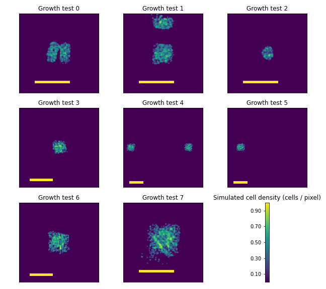
Figure C.2: The images in each plot show the simulated planar cell densities designed to match the experimental conditions shown in Figure C.1. Yellow scale bars in each image are 4mm.

Parameter fitting requires a generative model and a measure of goodness-of-fit between the simulated and experimental datasets. While the correspondence in spatiotemporal resolution of the two datasets encourage a measure that is a function of the residuals at each position and time, this was not the approach taken. The reason is that cell crowding and displacement are not features of the model. As the founding cells grow from single cells into microcolonies, they form expanding disks. Some of these disks remain within the bins used when performing downsampling while others do not. Increasing the downsampling scale factor reduces the impact of these bin-crossing microcolonies at the expense of spatial resolution. The scale factor of 64 was selected to reduce the impact cells passing into neighboring bins. However, there is another issue. Cells lose fluorescence as a result of loss-of-function mutations. Without the burden of expressing the reporter, mutant cells grow more rapidly than their neighbors and form large, expanding gaps in the fluorescence micrographs. This results both in vanishing cell density estimates within the mutant-occupied regions and crowding of fluorescent cells around the edges of these regions. If goodness-of-fit were calculated on a sum of residuals, it is likely that parameter inference routine would fit to these outlier data rather than overall distribution of growth rates.

To reduce the impact of loss-of-fluroescence mutants on parameter inference, the two-sample Kolmogorov-Smirnov goodness-of-fit function (K-S function) was used to compare the empirical distributions of the cell growth rates from the simulated and experimental data. The empirical cumulative distribution functions for the experimental and simulated datasets were calculated using 20 equal-width bins between growth rate values of 0 and 2 per hour. The K-S goodness-of-fit function \(f_{KS}\) used here to compare empirical cumulative density functions \(F_1\) and \(F_2\) describing samples of size \(p\) and \(q\) is \[\begin{equation} f_{KS}(F_1, F_2) = \frac{p\,q}{q+p} \mathrm{sup}_x | F_1(x) - F_2(x) | ^2 \end{equation}\] Cell growth rates were determined at each position and time by forward differences in cell densities. The parameter fitting routine used SciPy’s “optimize” module to find the parameter vector that minimized the K-S values, summed over each frame and growth context. While doing so eliminates the spatial information from the comparison, spatial variability in nutrient availability leads directly to shift of the empirical distribution of the growth rate towards slower growth. The K-S function therefore allows for parameter fitting in spite of obstacles presented by loss-of-function mutations and cell crowding.

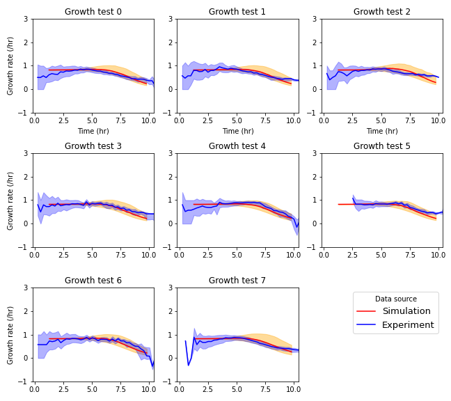
Figure C.3: Growth rate of cells in each growth context calculated by forward difference approximations. Simulation data was generated used the optimized parameter set. Solid lines represent mean growth rate, excepting empty positions. Shaded regions extend from the 25th to the 75th centile at each timepoint.

A comparison of the simulated behavior at best-fit parameters to experimental data are shown in Figure C.3. The clearest discrepancies are the wider distributions in growth rate seen in the simulated data as mean growth rate declines. However, the mean growth rates are very similar between datasets at all timepoints in all growth contexts.

References

Cao, Yangxiaolu, Marc D. Ryser, Stephen Payne, Bochong Li, Christopher V. Rao, and Lingchong You. 2016. “Collective Space-Sensing Coordinates Pattern Scaling in Engineered Bacteria.” Cell 165 (3): 620–30. https://doi.org/10.1016/j.cell.2016.03.006.

Liu, Chenli, Xiongfei Fu, Lizhong Liu, Xiaojing Ren, Carlos K. L. Chau, Sihong Li, Lu Xiang, et al. 2011. “Sequential establishment of stripe patterns in an expanding cell population.” Science 334 (6053): 238–41. https://doi.org/10.1126/science.1209042.

Payne, Stephen, Bochong Li, Yangxiaolu Cao, David Schaeffer, Marc D. Ryser, and Lingchong You. 2013. “Temporal control of self-organized pattern formation without morphogen gradients in bacteria.” Molecular Systems Biology 9 (1): 697. https://doi.org/10.1038/msb.2013.55.